Self Normalizing Flows
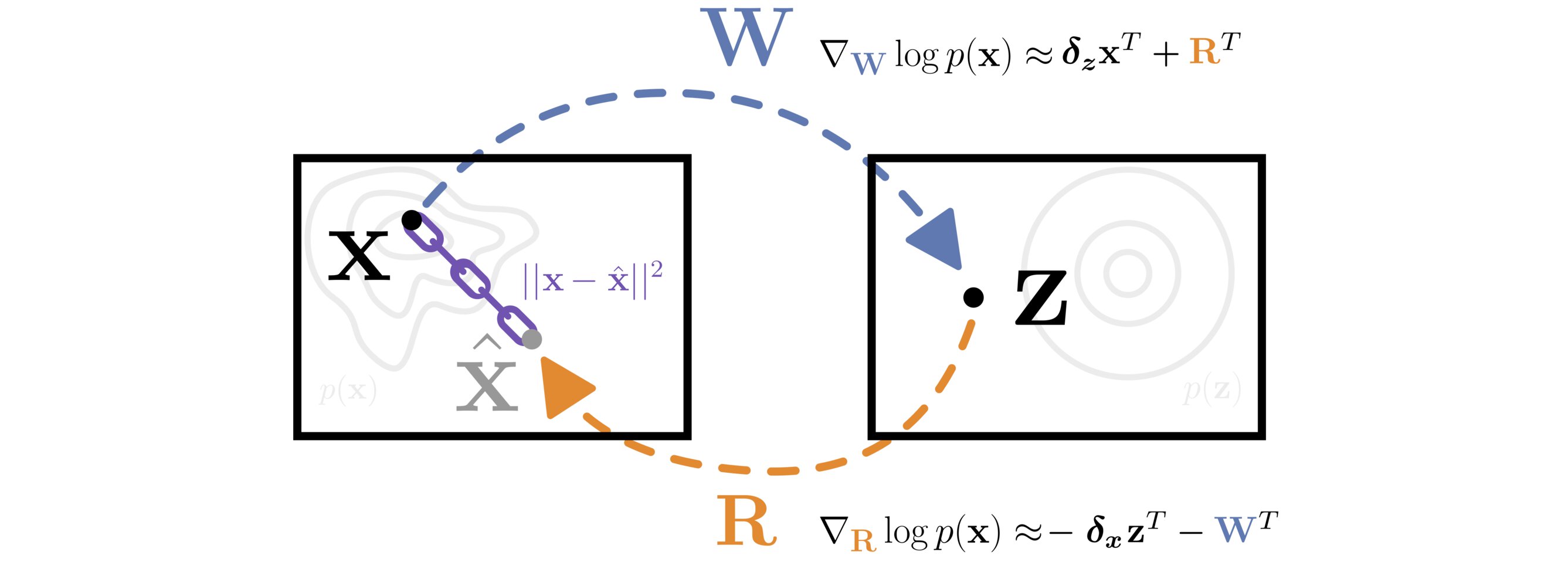 A matrix \(\mathbf{W}\) transforms data from \(\mathbf{X}\) to \(\mathbf{Z}\) space. The matrix \(\mathbf{R}\) is constrained to approximate the inverse of \(\mathbf{W}\) with a reconstruction loss \(||\mathbf{x} - \mathbf{\hat{x}}||^2\). The likelihood of the data is efficiently optimized with respect to both \(\mathbf{W}\) and \(\mathbf{R}\) by approximating the gradient of the log Jacobian determinant with the learned inverse.
Efficient gradient computation of the Jacobian determinant term is a core problem in many machine learning settings, and especially so in the normalizing flow framework. Most proposed flow models therefore either restrict to a function class with easy evaluation of the Jacobian determinant, or an efficient estimator thereof. However, these restrictions limit the performance of such density models, frequently requiring significant depth to reach desired performance levels. In this work, we propose Self Normalizing Flows, a flexible framework for training normalizing flows by replacing expensive terms in the gradient by learned approximate inverses at each layer. This reduces the computational complexity of each layer’s exact update from \(\mathcal{O}(D^3)\) to \(\mathcal{O}(D^2)\), allowing for the training of flow architectures which were otherwise computationally infeasible, while also providing efficient sampling. We show experimentally that such models are remarkably stable and optimize to similar data likelihood values as their exact gradient counterparts, while training more quickly and surpassing the performance of functionally constrained counterparts.
T. Anderson Keller, Jorn Peters, Priyank Jaini, Emiel Hoogeboom, Patrick Forré, Max Welling
ArXiv Paper: https://arxiv.org/abs/2011.07248
Accepted at: ICML 2021 and Beyond Backpropagation workshop at NeurIPS 2020
Github.com/akandykeller/SelfNormalizingFlows
- Video Summary
- Introduction
- Background
- Self Normalizing Flows
- Examples
- Results
- Discussion
- Example Implementation
Video Summary
Introduction
The goal of a probabilistic generative model is to accurately capture the true data generating process.1 Popular examples of such models include latent variable models (like Variational Autoencoders) or implicit probabilistic models (like Generative Adverserial Networks). In this work, we focus on another relatively recent technique for learning models of complex probability distributions – normalizing flows.
Normalizing flows are a powerful class of models which repeatedly apply simple invertible functions to transform basic probability distribtuions into complex target distributions. The primary goal of most work on normalizing flows is thus to develop new classes of functions which are simulatenously invertible, efficient to train, & maximally flexibile. For a complete and insightful review of normalizing flows, and prior work in this direction, I highly recommend reading Normalizing Flows for Probablistic Modeling and Inference (Papamakarios & Nalisnick et al. 2019).
In this work, we take a simple alternative approach which achieves the above three desired properties without having to resort to restriced function classes as prior work has done. We propose a new general framework called Self Normalizing Flows for the construction and training of normalizing flows which are virtually unconstrained (maximally flexible) while also being incredibly simple to train. Our work takes inspiration from ‘feedback’ connections observed in the biological cortex, and strives to simultaneously learn the inverse of each transformation performed in the flow.2 Our key insight is that the normally very expensive gradient update required to train the forward transformation is approximately given by the parameters of the learned inverse3 – thereby entirely avoiding the \(\mathcal{O}(D^3)\) computational complexity normally required for data of dimension \(D\).
Background
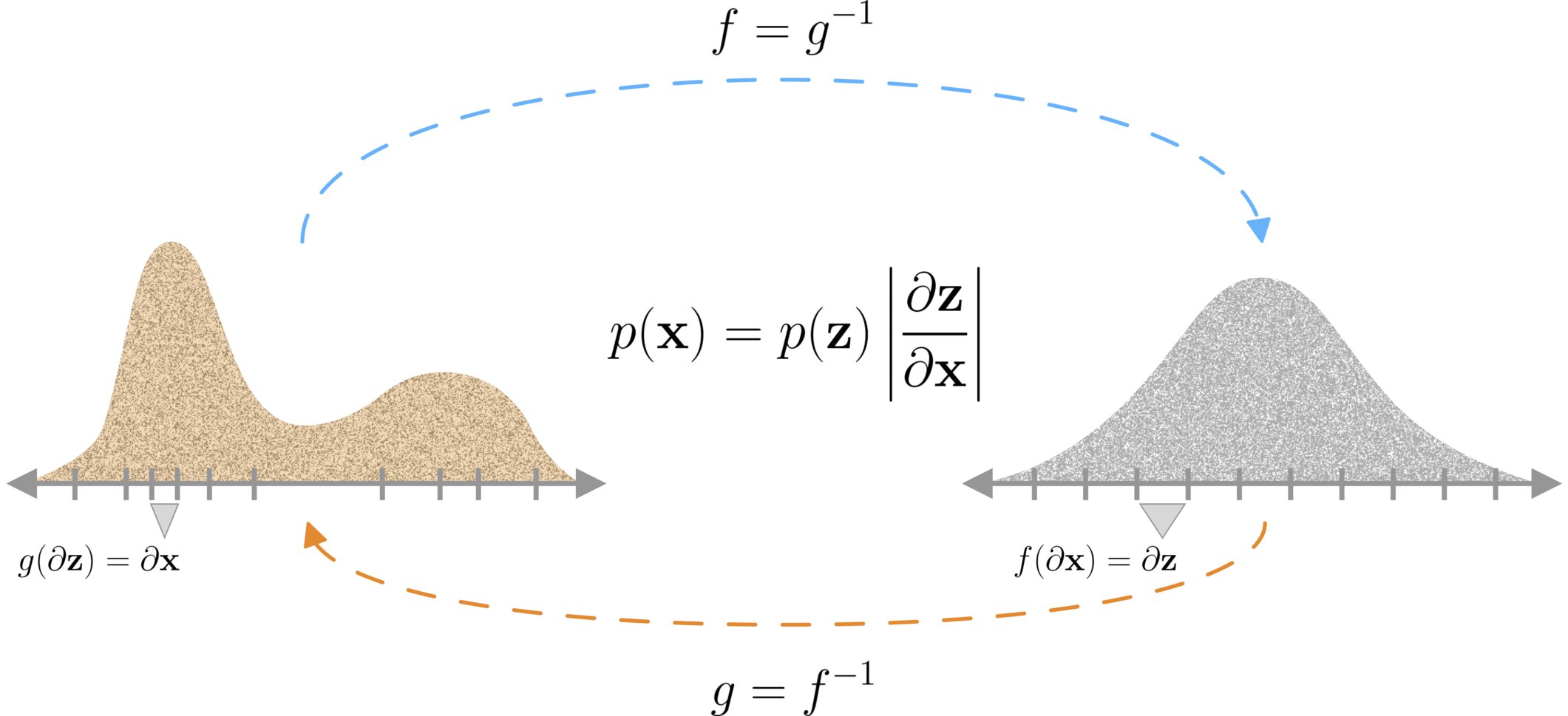
Given an observed data point \(\mathbf{x} \in \mathbb{R}^{D}\), it is assumed that \(\mathbf{x}\) is generated from an underlying (unknown) real vector \(\mathbf{z} \in \mathbb{R}^D\), through a ‘generating’ transformation \(g(\mathbf{z}) = \mathbf{x}\). In the normalizing flow framework, we assume that \(g\) is invertible, and we denote the inverse as \(f\), such that \(f = g^{-1}\) and \(f(\mathbf{x}) = \mathbf{z}\). Typically, normalizing flows are composed of many of such functions, i.e. \(g(\mathbf{z}) = g_K(g_{k-1}(\dots g_2(g_1(\mathbf{z}))))\), however in this blog post we will describe flows composed of a single ‘step’, since the proposed methods naturally extend to compositions.
The main idea behind normalizing flows is that since \(g\) is assumed to be a powerful transformation, we can transform from an easy to work with base distribution \(p_{\mathbf{Z}}\) (such as a Gaussian), to the true complex data distribution \(p_{\mathbf{X}}\), without having to know the data distribution directly. This transformation is achieved by the change of variables rule as follows:
$$ \begin{equation} \begin{split} p_{\mathbf{X}}(\mathbf{x}) & = p_{\mathbf{Z}}(\mathbf{z}) \left|\frac{\partial \mathbf{z}}{\partial\mathbf{x}}\right|\\ \Rightarrow p^g_{\mathbf{X}}(\mathbf{x}) & = p_{\mathbf{Z}}\left(g^{-1}(\mathbf{x})\right) \left|\mathbf{J}_{g^{-1}}\right| \\ \Rightarrow p^f_{\mathbf{X}}(\mathbf{x}) & = p_{\mathbf{Z}}\big(f(\mathbf{x})\big) \left|\mathbf{J}_f\right|\\ \end{split} \end{equation} $$
Where \(\left| \mathbf{J}_f \right| = \left|\frac{\partial f(\mathbf{x})}{\partial\mathbf{x}}\right|\) is the absolute value of the determinant of the Jacobian of the transformation between \(\mathbf{z}\) and \(\mathbf{x}\), evaluated at \(\mathbf{x}\). This term can intuitively be seen as accounting for the change of volume of the transformation between \(\mathbf{z}\) and \(\mathbf{x}\). In other words, it is the ratio of the size of an infinitesimally small volume around \(\mathbf{z}\) divided by the size of the corresponding transformed volume around \(\mathbf{x}\). We illustrate this simply with the following figure:
We see then, if we parameterize a function \(f_{\theta}\) with a set of parameters \(\theta\), and pick a base distribution \(p_{\mathbf{Z}}\), we can use the above equation to maximize the probability of observed data \(\mathbf{x}\) under our induced distributions \(p_{\mathbf{X}}^f(\mathbf{x})\).
Although in theory this allows us to exactly maximize the parameters of our model to make it a good model of the true data distribution, in practice, having to compute the Jacobian determinant \(\left|\mathbf{J}_f\right|\) or even it’s gradient \(\nabla_{\mathbf{J}_f} \left| \mathbf{J}_f \right| = \left(\mathbf{J}_f^{-1}\right)^T\) makes such an approach intractible for real data (both are \(\mathcal{O}(D^3)\) and consider even a small 256x256 image has over 65,000 dimensions).
Self Normalizing Flows
In this work, we take a different path than most normalizing flow literature, and instead of trying to simplify or approximate the computation of Jacobian determinant, we approximate its gradient. To do this, we leverage the inverse function theorem, which states that for invertible functions, the inverse of the Jacobian matrix is given by the Jacobian of the inverse function, i.e. \(\mathbf{J}_f^{-1} = \mathbf{J}_{f^{-1}}\). Thus, if we are able approximate the inverse of \(f\), we have simultaneously achieved an approximation for the gradient required to train \(f\). In other words, if \(f^{-1} \approx g\), then \(\mathbf{J}_{f}^{-1} \approx \mathbf{J}_{g}\), and we have avoided computation of both the inverse and the Jacobian determinant.4
Following this idea, we propose to define and parameterize both the forward and inverse functions \(f\) and \(g\) with parameters \(\theta\) and \(\gamma\) respectively. We then propose to constrain the parameterized inverse \(g\) to be approximately equal to the true inverse \(f^{-1}\) though a reconstruction loss. We can thus define our maximization objective as the mixture of the log-likelihoods induced by both models minus the reconstruction penalty constraint, i.e.:
$$\begin{equation} \begin{split} \mathcal{L}(\mathbf{x}) & = \frac{1}{2} \log p^{f}_{\mathbf{X}}(\mathbf{x}) + \frac{1}{2} \log p^{g}_{\mathbf{X}}(\mathbf{x}) - \lambda ||g \left( f (\mathbf{x}) \right) - \mathbf{x} ||^2_2 \end{split} \end{equation}$$
We see that when \(f = g^{-1}\) exactly, this is equivalent to the traditional normalizing flow framework.
Examples
Self Normalizing Fully Connected Layer
As a specific case of the above model, we consider a single fully connected layer, as exemplified in the figure at the top of this post. Let \(f(\mathbf{x}) = \mathbf{W} \mathbf{x} = \mathbf{z}\), and \(g(\mathbf{z}) = \mathbf{R} \mathbf{z}\), such that \(\mathbf{W}^{-1} \approx \mathbf{R}\). Taking the gradient of objective for this model, and approximating inverse matricies with their learned inverses, we get:
$$\begin{equation} \begin{split} \frac{\partial}{\partial \mathbf{W}} \mathcal{L}(\mathbf{x}) & = \frac{1}{2} \underbrace{\left(\frac{\partial}{\partial \mathbf{W}} \log p_{\mathbf{Z}}(\mathbf{W} \mathbf{x}) + \mathbf{W}^{-T}\right)}_{\textstyle \approx \delta_{\mathbf{z}} \mathbf{x}^T + \mathbf{R}^T} \ - \frac{\partial}{\partial \mathbf{W}} \lambda \mathcal{E} \end{split} \end{equation}$$ $$\begin{equation} \begin{split} \frac{\partial}{\partial \mathbf{R}} \mathcal{L}(\mathbf{x}) & = \frac{1}{2} \underbrace{\left(\frac{\partial}{\partial \mathbf{R}} \log p_{\mathbf{Z}}(\mathbf{R}^{-1} \mathbf{x}) - \mathbf{R}^{-T} \right)}_{\textstyle \approx - \delta_{\mathbf{x}} \mathbf{z}^T - \mathbf{W}^T}\ - \frac{\partial}{\partial \mathbf{R}} \lambda \mathcal{E} \\ \end{split} \end{equation}$$
where \(\mathcal{E}\) denotes the reconstruction error, \(\frac{\partial}{\partial \mathbf{W}} \lambda \mathcal{E} = 2\lambda \mathbf{R}^T(\hat{\mathbf{x}} - \mathbf{x}) \mathbf{x}^T\), \(\frac{\partial}{\partial \mathbf{R}} \lambda \mathcal{E} = 2\lambda (\hat{\mathbf{x}} - \mathbf{x})\mathbf{z}^T\), \(\hat{\mathbf{x}} = \mathbf{R}\mathbf{W}\mathbf{x}\), \(\delta_{\mathbf{z}} = \frac{\partial \log p_{\mathbf{Z}}(\mathbf{z})}{\partial \mathbf{z}}\), and \(\delta_{\mathbf{x}} = \frac{\partial \log p_{\mathbf{Z}}(\mathbf{z})}{\partial \mathbf{x}}\) are ordinarily computed by backpropagation. We observe that by using such a self normalizing layer, the gradient of the log-determinant of the Jacobian term is approximately given by the weights of the inverse transformation, sidestepping computation of the Jacobian determinant and all matrix inverses.
Self Normalizing Convolutional Layer
To construct a self normalizing convolutional layer, let \(f(\mathbf{x}) = \mathbf{w} \star \mathbf{x} = \mathbf{z}\), and \(g(\mathbf{z}) = \mathbf{r} \star \mathbf{z}\), such that \(f^{-1} \approx g\), where \(\star\) is the convolution operation. We first note that the inverse of a convolution operation is not necessarily another convolution. However, for sufficiently large \(\lambda\), we observe that \(f\) is simply restricted to the class of convolutions which is approximately invertible by a convolution. As we derive fully in the paper, the approximate self normalizing gradients with respect to a convolutional kernel \(\mathbf{w}\), and corresponding inverse kernel \(\mathbf{r}\), are given by: \[\begin{equation} \begin{split} \frac{\partial }{\partial \mathbf{w}} \log p^{f}_{\mathbf{X}}(\mathbf{x}) & \approx \delta_{\mathbf{z}} \star \mathbf{x} + \mathrm{flip}(\mathbf{r}) \odot \mathbf{m} \\ \end{split} \end{equation}\] \[\begin{equation} \begin{split} \frac{\partial }{\partial \mathbf{r}} \log p^{g}_{\mathbf{X}}(\mathbf{x}) & \approx -\delta_{\mathbf{x}} \star \mathbf{z} - \mathrm{flip}(\mathbf{w}) \odot \mathbf{m} \\ \end{split} \end{equation}\]
where \(\mathrm{flip}(\mathbf{r})\) corresponds to the kernel which achieves the transpose convolution and is given by swapping the input and output channels, and mirroring the spatial dimensions. The constant \(\mathbf{m}\) is given by the number of times each element of the kernel \(\mathbf{w}\) is present in the matrix form of convolution. The gradients for the reconstruction loss are then added to these to maintain the desired constraint.
Results
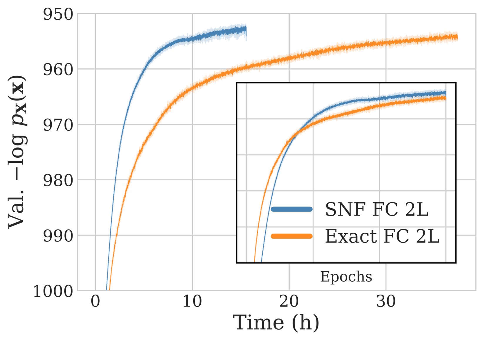
We evaluate our model by incorporating the above self normalizing layers into a variety of flow architectures and training them to maximize the proposed mixture objective on datasets including MNIST, CIFAR-10, and ImageNet32. We refer to the paper to see the full results and experiment details, but provide some highlights here. In the figure below, we show that a basic flow model composed of 2 self normalizing fully connected layers (SNF FC 2L) achieves similar (or better) performance than its exact gradient counterpart (Exact FC 2L), while training significantly faster.
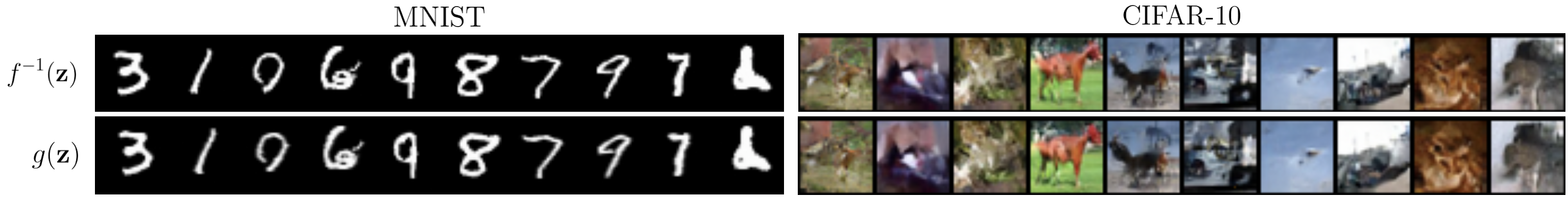
We can additionally see that samples from the model appear to match samples from the true data distribution. In the figure below, we show samples from \(p_{\mathbf{Z}}\) passed through both the true inverse \(\mathbf{x} = f^{-1}(\mathbf{z})\) (top) and the learned inverse \(\mathbf{x} = g(\mathbf{z})\) (bottom). We see that the samples are virtually indistinguishable, thus implying that the model has learned to approximate its own inverse well, while simultaneously learning a good model of the data distribution (since the samples look like realistic images).
Discussion
We see that the above framework yields an efficient update rule for flow-based models which appears to perform similarly to the exact gradient while allowing for the training of flow architectures which were otherwise computationally infeasible. We believe this opens up a broad range of new research directions involving less constrained flows, and intend to investigate such directions in future work. Furthermore, we believe the biological motivation and plausibility of this model are also worth exploring further. Ideally, we believe the gradient approximation used here could be combined with backpropagaion-free training methods such as Target Propagation, allowing for a fully backprop-free unsupervised density model.
Example Implementation
Below we give an example implementation of the above convolutional layer in Pytorch (which is also a generalization of the fully connected layer). We make use of the pytorch autograd API to create a fast and modular implementation. We note that this implementation still requires the layer-wise reconstruction gradients to be computed and added to this separately. The full code for the paper is available at the repository here: github.com/akandykeller/SelfNormalizingFlows
class SelfNormConvFunc(autograd.Function):
    @staticmethod
    def forward(ctx, x, W, bw, R, stride, padding, dilation, groups):
        z = F.conv2d(x, W, bw, stride, padding, dilation, groups)

        ctx.save_for_backward(x, W, bw, R, z)
        ctx.stride = stride
        ctx.padding = padding
        ctx.dilation = dilation
        ctx.groups = groups
        return z

    @staticmethod
    def backward(ctx, output_grad):
        x, W, bw, R, output = ctx.saved_tensors

        stride = torch.Size(ctx.stride)
        padding = torch.Size(ctx.padding)
        dilation = torch.Size(ctx.dilation)
        groups = ctx.groups
        benchmark = False
        deterministic = False

        multiple = _compute_weight_multiple(W.shape, output, x, padding, stride,
                            dilation, groups, benchmark, deterministic)

        # Grad_W LogP(x)
        delta_z_xt = conv2d_backward.backward_weight(W.shape, output_grad, x,
                                                     padding, stride, dilation,
                                                     groups, benchmark, deterministic)
        weight_grad_fwd = (delta_z_xt - flip_kernel(R) * multiple) / 2.0

        # Grad_R LogP(x)
        input_grad = conv2d_backward.backward_input(x.shape, output_grad, W,
                                                    padding, stride, dilation,
                                                    groups, benchmark,
                                                    deterministic)
        Wx = output - bw.view(1, -1, 1, 1) if bw is not None else output
        neg_delta_x_Wxt = conv2d_backward.backward_weight(W.shape, -1*input_grad, Wx,
                                                          padding, stride, dilation,
                                                          groups, benchmark,
                                                          deterministic)
        weight_grad_inv = (neg_delta_x_Wxt + flip_kernel(W) * multiple) / 2.0

        if bw is not None:
            # Sum over all except output channel
            bw_grad = output_grad.view(output_grad.shape[:-2] + (-1,)).sum(-1).sum(0)
        else:
            bw_grad = None

        return input_grad, weight_grad_fwd, bw_grad, weight_grad_inv, None, None, None, None
The above code requires the use of pytorch’s autograd functions backward_weight and backward_input. The pytorch implementations can be found here, however, these are much slower than the C++ implementations. To use the C++ implementations, we built a simply torch C++ extension. Please see the full repository for reference.
Finally, the above code makes use of two helper functions to compute the multiple, and ‘flip’ the kernel, these functions can be implemented as:
@lru_cache(maxsize=128)
def _compute_weight_multiple(wshape, output, x, padding, stride, dilation,
                                 groups, benchmark, deterministic):
    batch_multiple =  conv2d_backward.backward_weight(wshape,
                                           torch.ones_like(output),
                                           torch.ones_like(x),
                                           padding, stride, dilation,
                                           groups, benchmark, deterministic)
    return batch_multiple / len(x)


def flip_kernel(W):
    return torch.flip(W, (2,3)).permute(1,0,2,3).clone()
Similarly, the goal of probabilistic generative models can be seen as designing models which are able to generate data which appears to come from the same distribution as real data. ↩︎
Or equivalently, learn the inverse of each layer. We note that we are far from the first to propose this idea. The works of Difference Target Propagation, and (Rippel and Adams 2013) both use similar learned inverses at each layer for different purposes, just to name a few. Our work however, is the first to our knowledge to propose using the learned inverse as a direct approximation to computaionally expensive gradients. Please see the full paper for a full overview of related work. ↩︎
The gradient is given exaclty by the inverse parameters only in the case of linear transformations (since in this case the Jacobian of the transformation is equal to the linear map itself). For non-linear self normalizing flows we direct the reader to the general framework of our paper, where the Jacobian of the inverse transformation is used in-place of the inverse of the Jacobian of the forward transformation. ↩︎
This assumes that \(f^{-1} \approx g\) implies \(\mathbf{J}_{f^{-1}} \approx \mathbf{J}_g\). We note that this is true for all linear functions \(f\), but may not be true for certain high frequency functions. In such cases, we propose the penalize the jacobians to be approximately equal directly. ↩︎